When it comes to attacker infrastructure, some threats are more stealthy than others. Searching “cobalt strike beacon” in Shodan or similar tools can reveal exposed Teams Servers that are not properly protected from the public eye – as shown below.
Example Cobalt Strike beacon configuration results from Shodan
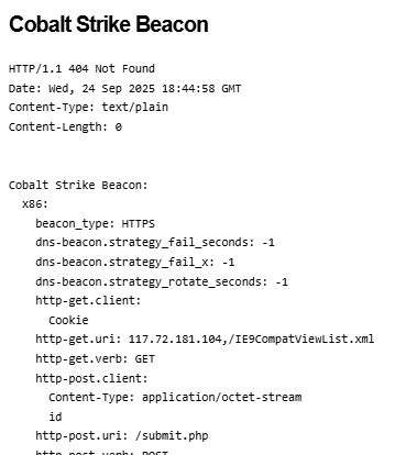
Additionally, these servers often expose details of configured beacon behavior that can be used to study how attackers are setting up initial payload functionality – an example is shown below.
Example beacon configuration screenshot from Shodan
These types of details are invaluable and allow us to study the settings attackers are using for their Cobalt Strike payloads – often these carry over into other frameworks as well such as Sliver, Mythic, etc. In this post, I present a statistical summary of beacons exposed at the time of this writing to help suggest detection and hunting ideas for blue teams.
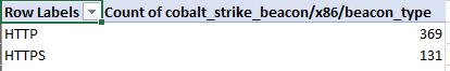
One of the most obvious things we can look at first is understanding the type of beacons that threat actors are using – Cobalt Strike supports a variety of types including HTTP, HTTPS and DNS – threat actors today typically use HTTPS, as evidenced in the below analysis (with DNS being exceedingly rare due to how slow they are to interact with).
Cobalt Strike Beacon Types
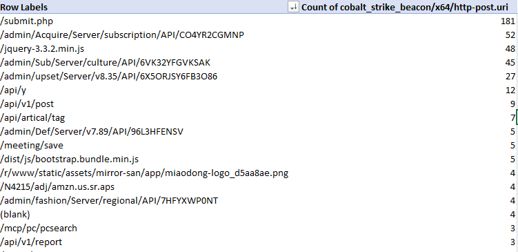
When threat actors are setting up an HTTP-based beacon, they must configure different properties such as the URIs that will be invoked, the user agent, the HTTP verbs, etc – so let’s take a look at these – starting with the most common POST URIs setup by actors.
Most common POST URIs for Beacons
A couple of these standout – threat actors really like ‘submit.php’, URIs that appear to be API endpoints and URIs that look like common web-app behavior such as loading jquery. This is good material for pivoting using other material to find potential C2 behavior in your network.
Looking at sleeptime also exposes some interesting data – the vast majority of exposed configurations used the default sleeptime setting of 60 seconds – the next biggest bucket of actors reduced this to 3 seconds – then we can observe a variety of different configurations.
Sleep Time configurations from Beacons – Sleep Time on the left, count of appearances on the right
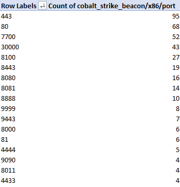
In terms of TCP Ports, we observe beacons communicating on a wide variety of outbound connections. In my experience doing Incident Response, C2 traffic tends to stick to port 80 or 443 but this is evidence that this is not always the case!
Most common ports for beacon configurations
The above image shows only the most common ports in use – there were dozens of other ports not pictured that were used by 3 or less observed configurations.
What about the HTTP user agent in use? There was a significant amount of variety here (as expected), with configurations trying to impersonate various browsers and devices such as iPads, Mac OS, Windows, etc. The most commonly observed ones are shown below.
Most common User Agents observed in configurations
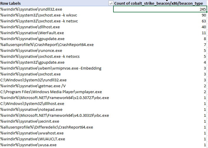
Let’s now analyze the characteristics of beacon process spawning and injection behavior. Cobalt Strike enables operators to configure ‘post exploitation’ configurations that control how sub-processes are spawned from a primary beacon. The table below represents the binaries that were configured for use with post-exploitation tasks such as screenshots, key-logging, scanning, etc.
x86 spawn_to configurations for Cobalt Strike beacons
As we can see, the most common choice by far was rundll32.exe, followed by svchost.exe, dllhost.exe, WerFault.exe and gpuupdate.exe – but there are definitely some less-observed binaries in the table. I would urge defenders to ensure you are considering all possible hunting options when looking for C2 traffic in your network.
There are many additional aspects of Cobalt Strike configurations that we as blue-teamers can pivot and hunt on throughout our networks – the goal of this is to help shine some light on the most commonly used and abused components so that hunt and detection teams can embrace these attributes and improve their security posture. My hope is that you can immediately take some of these data points and action them internally on your own network for finding suspicious activity, should it exist.
I’ll continue this analysis in an additional post as I dive into other C2 servers and additional discovery mechanisms for Cobalt Strike servers, among other platforms.
Recently I’ve been wanting to dive into anomaly detection and classification problems – I’m starting this by exploring a binary-classification issue – trying to determine whether or not a PowerShell snippet is benign or suspicious.
There are many different approaches to this problem-class. I decided to start with a “batteries-included” approach to text classification with the help of fastText (https://github.com/facebookresearch/fastText). This awesome piece of software from Facebook Research can perform both un-supervised and supervised training with tunable parameters on a set of pre-processed input data.
Similar to most other data science projects, I started this by spending a significant amount of time identifying and categorizing source material, mostly by scraping PowerShell scripts available from a variety of sources (e.g., GitHub, Hybrid Analysis, etc). Each script was saved into a labelled directory indicating what type of scripts it contains. Since this is a binary classification task, we are only going to be using the labels of ‘suspicious’ or ‘benign’ with each script having exactly 1 label.
A future task would be adding additional labels such as “malicious” to provide more flexibility to the classifications and subsequent conclusions we draw from them (I stored them with some flexibility to distinguish between suspicious and purely malicious but am only using the single label of ‘suspicious’ for this experiment).
Example showing data organization / classification structure
Another approach to this problem would be creating many different distinct labels and using the percent confidence for each to infer what the functionality of the script is, what MITRE Techniques it is employing, etc.
Text Classification with fastText
Supervised Learning with fastText for Text Classification can be done by supplying the model with an input file in a specific format. The default structure should contain line-delimited data where lines begin with all relevant labels for the current line. The default format for labels is ‘__label__$VAR’ where $VAR is the relevant key-word such as ‘__label__benign’.
__label__benign some line of data
__label__suspicious another line of data
For this experiment, I wanted to try a few different methods of classifying scripts. Initially, I did a very basic implementation to try a pure text classification approach. Later on, I’d like to combine this model’s prediction output with an Abstract Syntax Tree (AST) neural network analysis to produce a combined probability matrix ,which we can then analyze to more effectively determine if a script is suspicious or not.
For now, I took the following approach to data preparation;
Read each script into memory
Normalize the data by stripping white-space and lower-casing the entire script
Remove un-wanted characters to help improve classification traits
Write each script (as a single string per-line) into a file with the relevant label as a prefix
After this initial data aggregation step, I shuffled the line-ordering and split the data into a 70/30% mix of training and test data respectively. Using 100% of the source data to train can overfit a model to the training data and lead to critical failures when classifying new data – this helps identify that problem and attempt to mitigate early on.
Total Scripts: 10433
Training Data Length: 7303
Testing Data Length: 3130
Suspicious Scripts: 4776
Benign Scripts: 5657
Now it’s time for the fun part. Training a fastText model can have a lot of nuances but at it’s core, it can be done in two lines like this.
import fasttext
model = fasttext.train_supervised('pslearn.train')
That’s it! – I can now use the test dataset to gauge the prediction accuracy of our first supervised fastText model.
The first number (3130) represents the number of samples in the test data. The second number represents the precision (~94%) and the last number represents the recall (~94%).
Per fastText documentation:
The precision is the number of correct labels among the labels predicted by fastText. The recall is the number of labels that successfully were predicted, among all the real labels.
A precision metric of 94% seems extremely high – I have a very limited sample set and it is highly likely that I have accidentally introduced a high amount of bias to the source data. One way I can solve this is by reviewing the data and ensuring that there is a wide variety of samples in different formats and stylings to introduce additional variety to the training and testing data.
For now, lets see if I can improve the model by using some additional options provided by fastText – word n-grams and epoch count. By default, fastText only uses 5 epochs for learning – lets try tripling that number to 15 and see if there is any effect on the accuracy.
model = fasttext.train_supervised('pslearn.train', epoch=15)
model.test('pslearn.test')
(3130, 0.9619808306709265, 0.9619808306709265)
A small increase in the number of epochs had a significant effect on the accuracy, however, the trade-off is a longer processing time when training (or re-training) the model. Since we have a relatively small data set (~100 MB) I can experiment with extremely high epoch counts such as 1000+, like below.
model = fasttext.train_supervised('pslearn.train', epoch=1000)
model.test('pslearn.test')
(3130, 0.9769968051118211, 0.9769968051118211)
The key to data science is always experimentation – I played with the epoch count for a while to find the optimal balance of time to run vs accuracy vs not overfitting to the current data. At 500 runs I still had a precision measurement of 97.6%, 250 runs actually increased to 98% while 100 lowered slightly to 97.8% – 50 runs achieved an accuracy of 97.5%, and 25 runs was 96.9%. I decided to keep it at 25 to avoid overfitting for most of this experiment.
In addition to epoch count, one of the other commonly tuned parameters for a fastText model is the learning rate. For a detailed explanation, check out the documentation at https://fasttext.cc/docs/en/supervised-tutorial.html. The default Learning Rate is 0.1, but lets try 0.2 and see if there is any improvement when using an epoch count of 25.
model = fasttext.train_supervised('pslearn.train', epoch=25, lr=0.2)
model.test('pslearn.test')
(3130, 0.9750798722044729, 0.9750798722044729)
Doubling the learning rate improved our base accuracy at 25 epochs from ~96.9% to ~97.5%.
Word N-Gram length should be decided based on the current use-case as well as experimented with since it can have a severe impact on model accuracy depending on the type of data. I decided to leave it at the default for now.
Below you can see the results of some of the ad-hoc tests I ran against it with some arbitrary PowerShell scripts that were not included in testing or training data.
No, not really – I have a really small sample set of data and it is highly biased. I also don’t have many ‘real world’ samples right now but am working on a pipeline to generate more variants like you might expect to see in a true adversary engagement. As per above, this type of ‘simple’ text classification can work but is very lacking when it comes to highly-complex use-cases where the same ‘sentiment’ can be expressed in hundreds of ways – what else can I do?
Embed additional labelling for each script to help with classifying and having a secondary process for guessing probability based on the confidence in each label
Gather/Generate additional source data for better classification and a wider variety of training and testing data
Experiment with different text classification models
etc
Using fastText itself is ridiculously easy – the hard part of a data scientists life is preparing the source material. Data Pre-Processing pipelines are often extremely complex to ensure the cleanest feed to downstream ML models – the exact type of processing required is typically dependent on project-specific features such as the overall objective, the types of machine-learning models or approaches, etc.
AST Modeling in a Deep Neural Network (DNN)
In addition to text classification, I wanted to try feature engineering for a machine-learning model. Ultimately, I decided to use my features inside of a “Deep & Wide” style network built with Keras and Tensorflow. Feature Engineering is probably one of the most important part of any ML workflow – for this project, I took a basic approach and using https://github.com/thewhiteninja/deobshell I generated optimized AST files for each of the previously collected PowerShell scripts.
In generating features from these ‘optimized’ AST representations we can parse the script functionality at a lower-level than just reading the raw .ps1 file and receive more meaningful insight into what components make up the script.
Why would I want to do this? fastText is great but studying the data at a lower-level in a neural network could help teams gain some deeper insight into the data in a way that fastText might not help us as much with. Ultimately, the best approach would be to have multiple prediction pipelines to get outputs from various models and glue the results together with some logic.
I parsed each AST and generated a set of features representing the below items (along with a few others)
Distinct PowerShell Tree-Type Count
Sum for each type of AST Object present in the script (CommandElementAST, etc)
Variable / Operator / Condition sums
Presence of certain ‘suspicious’ strings inside the script (‘IEX’, etc)
etc
Once I have the data cleaned and stored appropriately in a CSV, I can set up the below workflow for running independent experiments (code truncated for readability).
# Setup Required Imports, Constants, etc
CSV_HEADER = []
NUMERIC_FEATURE_NAMES = []
for c in raw_data.columns:
    CSV_HEADER.append(c)
    if c != 'label':
        NUMERIC_FEATURE_NAMES.append(c)

# All of my features are numeric and not categorical
TARGET_FEATURE_NAME = "label"
TARGET_FEATURE_LABELS = [0.0, 1.0]
CATEGORICAL_FEATURES_WITH_VOCABULARY = {}
CATEGORICAL_FEATURE_NAMES = list(CATEGORICAL_FEATURES_WITH_VOCABULARY.keys())
FEATURE_NAMES = NUMERIC_FEATURE_NAMES + CATEGORICAL_FEATURE_NAMES
COLUMN_DEFAULTS = [[0.0] for feature_name in CSV_HEADER]
NUM_CLASSES = len(TARGET_FEATURE_LABELS)

# How the model will parse the data from disk
def get_dataset_from_csv(csv_file_path, batch_size, shuffle=False):
    dataset = tf.data.experimental.make_csv_dataset(
        csv_file_path,
        batch_size=batch_size,
        column_names=CSV_HEADER,
        column_defaults=COLUMN_DEFAULTS,
        label_name=TARGET_FEATURE_NAME,
        num_epochs=1,
        header=True,
        shuffle=shuffle,
    )
    return dataset.cache()

# Invoke an experiment
def run_experiment(model):
    model.compile(
        optimizer=keras.optimizers.Adam(learning_rate=learning_rate),
        loss=keras.losses.SparseCategoricalCrossentropy(),
        metrics=[keras.metrics.SparseCategoricalAccuracy()],
    )
    train_dataset = get_dataset_from_csv(train_data_file, batch_size, shuffle=True)
    test_dataset = get_dataset_from_csv(test_data_file, batch_size)
    print("Start training the model...")
    history = model.fit(train_dataset, epochs=num_epochs)
    print("Model training finished")
    _, accuracy = model.evaluate(test_dataset, verbose=0)
    print(f"Test accuracy: {round(accuracy * 100, 2)}%")

# Encode Input Layers
def create_model_inputs():
    return inputs

# Encode Features depending on type
def encode_inputs(inputs, use_embedding=False):
    return all_features

# Create Keras Network Model - using a softmax output
def create_wide_and_deep_model():
    return model

# Run the experiment!
wide_and_deep_model = create_wide_and_deep_model()
#keras.utils.plot_model(wide_and_deep_model, show_shapes=True, rankdir="LR")
run_experiment(wide_and_deep_model)

Start training the model...
Epoch 1/10
32/32 [==============================] - 453s 3s/step - loss: 0.4908 - sparse_categorical_accuracy: 0.7793
Epoch 2/10
32/32 [==============================] - 8s 239ms/step - loss: 0.2756 - sparse_categorical_accuracy: 0.9325
Epoch 3/10
32/32 [==============================] - 8s 245ms/step - loss: 0.2000 - sparse_categorical_accuracy: 0.9508
Epoch 4/10
32/32 [==============================] - 8s 244ms/step - loss: 0.1548 - sparse_categorical_accuracy: 0.9580
Epoch 5/10
32/32 [==============================] - 8s 245ms/step - loss: 0.1358 - sparse_categorical_accuracy: 0.9640
Epoch 6/10
32/32 [==============================] - 8s 249ms/step - loss: 0.1196 - sparse_categorical_accuracy: 0.9656
Epoch 7/10
32/32 [==============================] - 8s 246ms/step - loss: 0.1073 - sparse_categorical_accuracy: 0.9671
Epoch 8/10
32/32 [==============================] - 8s 245ms/step - loss: 0.0965 - sparse_categorical_accuracy: 0.9695
Epoch 9/10
32/32 [==============================] - 8s 243ms/step - loss: 0.1022 - sparse_categorical_accuracy: 0.9666
Epoch 10/10
32/32 [==============================] - 8s 244ms/step - loss: 0.0940 - sparse_categorical_accuracy: 0.9711
Model training finished
Test accuracy: 74.9%
In the end, I can see the network was able to predict whether a script in the validation data was suspicious or not with a ~75% accuracy – not too bad for the very first attempt. Doubling the epoch count to 20 runs got me to ~80% accuracy without a huge risk of over-fitting. What else could I do to improve this?
Feature Dimensionality Reduction (Linearly with PCA or non-linearly with better AutoEncoders)
Better Feature Engineering – it is very basic currently
Tuning Model Parameters/Hyperparameters manually to experiment with learning impact
I have some other ideas for feature building techniques with respect to PowerShell analysis that I’m excited to keep exploring and building machine-learning models around – if you’re interested in similar topics, reach out and lets discuss!
Machine Learning to identify evil isn’t a new concept – but the exact techniques utilized are not often shared to the public for a few reasons. First being that threat actors could analyze then workaround the detection mechanisms and secondly, these workflows often power revenue-generating streams and sharing them could impact profits. I’m hoping that in coming years the open-source detection community starts to build and share more ready-to-use models that organizations can use for these types of classification tasks.
Look out for the next post, should be interesting – and let me know if there are any questions!