While doing some pivoting on emerging Command and Control servers, I identified an open-directory on an IP Address (144.31.106[.]169) hosting what appeared to be a collection of malicious shell scripts, as shown below.
Initial Open Directory Contents
Contents of ‘stagers’ directory
Peering into the first shell script, ‘mimicry.sh’, its purpose appears to be serving as a staging script for the actual payload – ocean_strike_v5.tar.gz – curling the payload into /tmp/.sys-task, extracting it, starting a secondary shell script, then deleting the previously created directory. Let’s take a look inside ocean_strike_v5.tar.gz.
mimicry.sh
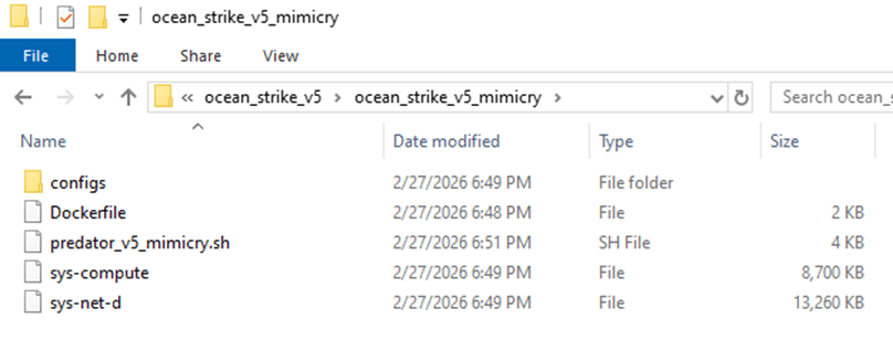
ocean_strike_v5 contents
The script of interest, ‘predator_v5_mimicry.sh’, is a shell script designed to perform the following actions:
Checks if it is running insider a container, sandbox, WSL, or other virtualization environment using /proc/1/cgroup
Adds an SSH key to /root/.ssh/authorized_keys to maintain persistent access to the compromised device
Attempts to set vm.nr_hugepages=1280 – increasing performance of certain workloads, including crypto-mining
Attempts to identify any other mining-related processes and kill them, including anything that mentions guard, miner, YDServi, xmrig, nanominer, kdevtmpfsi, gost, pcpcat, or proxy.sh
Creates directory /dev/shm/.sys-cache and copies some of the above files into it – sys-compute is copied as kworker and made executable.
A service is also installed named ‘System Monitoring Service’ to ensure it is always running.
The malware then configures what it refers to as a Mimicry Proxy via the binary sys-net-d seen above – this is installed into /usr/bin/sys-net-d with a service setup named ‘Network Monitoring Service’.
The malware then attempts to build something it refers to as a ‘Mimicry Aquarium’ using the contained docker file, spawning a container named ‘sys-aquarium-mimicry’ and mapping host port 2376 to container port 2375.
The container appears intended to serve as a distraction for other attackers – it installs some common Linux utilities such as curl, wget, etc, creates fake artifacts like /root/proxy.sh, creates a cron job without actually enabling it to run proxy.sh every 30 minutes, then creates an empty file at /var/run/docker.sock
The container itself is used to return a general HTTP 200 Status in response to any request to port 2375, the Docker Remote API.
The attacker then uses iptables to redirect any inbound request destined for port 2375 to port 2376 – effectively capturing traffic destined for the Docker Remote API into the container, which then supplies a ‘fake’ response.
This is done seemingly to prevent any additional tampering or exploitation from occurring that may interfere with their mining services.
Their own IP address is excluded from this port mapping rule via iptables
Finally, the attacker writes to a file called /dev/shm/.sys-cache/watchdog.sh a bash script that periodically wakes and checks 144.31.106[.]169 for a 200 OK response – if it is not received, it clears all iptables pre-routing and restarts the main docker service.
This is to ensure access to the true Docker API port is available remotely again for a potential re-compromise
In total, the malware attempts to find and kill competitors, deploys persistence via system services, runs a Docker container to proxy traffic to the Remote Docker API port, deploys a crypto-miner onto the device, and implements a dead mans switch designed to clear the routing trap should the main IP address fail to respond.
Dead Mans Switch in predator_v5_mimicry.sh
After some research, I reached the following conclusions:
sys-net-d appears to be a Sliver agent payload (tracks with Sliver C2 exposed on the IP address already).
sys-compute is an XMRig mining binary, avoiding the overhead of having to download it dynamically on victim systems.
While digging into other directories, I found multiple older versions of their persistence and deployment scripts along with potential targets in the ‘ocean_strike.tar.gz’ file, as shown below:
Contents of ocean_strike.tar.gz
The observed sys-net-d and sys-compute are the same Sliver payload and XMRig binary previously noted. There are variations of persistence scripts present, but all ‘deployer’ scripts are 0-byte files as of the time of this analysis. Sys-guard is a simple shell script that configures ocean-miner along with a decoy Docker container, another variation of Monero mining.
What’s more interesting is the files labelled ‘fortress_results’ – these appear to be scans of potential victim IP addresses – each victim had an exposed Remote Docker API port that the threat actor tested to determine the level of access they could achieve remotely, attempting to create a privileged container to facilitate mining operations.
fortress_results_v2 demonstrating attempts to create privileged containers on exposed Docker instances across the Internet on a variety of victim networks
Revisiting one of the earlier files, we identified another Monero miner staging script named ‘cuckoo_stager.sh’. This is similar to the ‘Ocean Strike’ payload but had slightly different checks for containers, competitors, deployment, persistence, and fail-over operations. A snippet is shown below.
cuckoo_stager.sh snippet
In essence, this script attempted to:
Identify if it’s in a container via the presence of ‘docker’ in /proc/1/cgroup and also checking for the presence of systemd
Kill other competing mining processes
Download xmrig and Yggdrasil payloads binaries from the main control address (144.31.106[.]169)
Configure and launch xmrig for Monero mining
Persist itself via cron jobs
Hide initial access by deleting bash history and timestomping xmrig binary and configuration files to appear older than they are
Delete the initial stager (/tmp/cuckoo_stager.sh)
Then, optionally, starting Yggdrasil mesh network in an attempt to obfuscate traffic destinations and avoid initial detection at the network level
There was a final script named ‘dead_man_switch.sh’ that appears similar in nature to the fallback utilized in the original ‘Ocean Strike’ script in that it periodically checks if a specific heartbeat is being populated – if no heartbeat is detected after a 30 minute period, it assumes there is a catastrophic error with the script and attempts to re-expose the original Docker API ports instead of the mimicked port so that remote access can once again be gained by the actor.
dead_man_switch.sh snippet
Conclusions
This is an interesting malware variant that is explicitly targeting the Remote Docker API in an attempt to create high-privileged containers on exposed ports that are then leveraged to instantiate Monero-mining operations – this is not a new technique, but it is still interesting from a defensive perspective to study the source and implementation so that we can further harden relevant systems.
Once the malware is deployed, the Docker API port (2375) is then proxied to 2376 via a ‘decoy’ container and iptables, likely to ensure that other actors cannot launch competing resources – but in such a way that the C2 IP address can still reach the original port without interference.
Recently I’ve been wanting to dive into anomaly detection and classification problems – I’m starting this by exploring a binary-classification issue – trying to determine whether or not a PowerShell snippet is benign or suspicious.
There are many different approaches to this problem-class. I decided to start with a “batteries-included” approach to text classification with the help of fastText (https://github.com/facebookresearch/fastText). This awesome piece of software from Facebook Research can perform both un-supervised and supervised training with tunable parameters on a set of pre-processed input data.
Similar to most other data science projects, I started this by spending a significant amount of time identifying and categorizing source material, mostly by scraping PowerShell scripts available from a variety of sources (e.g., GitHub, Hybrid Analysis, etc). Each script was saved into a labelled directory indicating what type of scripts it contains. Since this is a binary classification task, we are only going to be using the labels of ‘suspicious’ or ‘benign’ with each script having exactly 1 label.
A future task would be adding additional labels such as “malicious” to provide more flexibility to the classifications and subsequent conclusions we draw from them (I stored them with some flexibility to distinguish between suspicious and purely malicious but am only using the single label of ‘suspicious’ for this experiment).
Example showing data organization / classification structure
Another approach to this problem would be creating many different distinct labels and using the percent confidence for each to infer what the functionality of the script is, what MITRE Techniques it is employing, etc.
Text Classification with fastText
Supervised Learning with fastText for Text Classification can be done by supplying the model with an input file in a specific format. The default structure should contain line-delimited data where lines begin with all relevant labels for the current line. The default format for labels is ‘__label__$VAR’ where $VAR is the relevant key-word such as ‘__label__benign’.
__label__benign some line of data
__label__suspicious another line of data
For this experiment, I wanted to try a few different methods of classifying scripts. Initially, I did a very basic implementation to try a pure text classification approach. Later on, I’d like to combine this model’s prediction output with an Abstract Syntax Tree (AST) neural network analysis to produce a combined probability matrix ,which we can then analyze to more effectively determine if a script is suspicious or not.
For now, I took the following approach to data preparation;
Read each script into memory
Normalize the data by stripping white-space and lower-casing the entire script
Remove un-wanted characters to help improve classification traits
Write each script (as a single string per-line) into a file with the relevant label as a prefix
After this initial data aggregation step, I shuffled the line-ordering and split the data into a 70/30% mix of training and test data respectively. Using 100% of the source data to train can overfit a model to the training data and lead to critical failures when classifying new data – this helps identify that problem and attempt to mitigate early on.
Total Scripts: 10433
Training Data Length: 7303
Testing Data Length: 3130
Suspicious Scripts: 4776
Benign Scripts: 5657
Now it’s time for the fun part. Training a fastText model can have a lot of nuances but at it’s core, it can be done in two lines like this.
import fasttext
model = fasttext.train_supervised('pslearn.train')
That’s it! – I can now use the test dataset to gauge the prediction accuracy of our first supervised fastText model.
The first number (3130) represents the number of samples in the test data. The second number represents the precision (~94%) and the last number represents the recall (~94%).
Per fastText documentation:
The precision is the number of correct labels among the labels predicted by fastText. The recall is the number of labels that successfully were predicted, among all the real labels.
A precision metric of 94% seems extremely high – I have a very limited sample set and it is highly likely that I have accidentally introduced a high amount of bias to the source data. One way I can solve this is by reviewing the data and ensuring that there is a wide variety of samples in different formats and stylings to introduce additional variety to the training and testing data.
For now, lets see if I can improve the model by using some additional options provided by fastText – word n-grams and epoch count. By default, fastText only uses 5 epochs for learning – lets try tripling that number to 15 and see if there is any effect on the accuracy.
model = fasttext.train_supervised('pslearn.train', epoch=15)
model.test('pslearn.test')
(3130, 0.9619808306709265, 0.9619808306709265)
A small increase in the number of epochs had a significant effect on the accuracy, however, the trade-off is a longer processing time when training (or re-training) the model. Since we have a relatively small data set (~100 MB) I can experiment with extremely high epoch counts such as 1000+, like below.
model = fasttext.train_supervised('pslearn.train', epoch=1000)
model.test('pslearn.test')
(3130, 0.9769968051118211, 0.9769968051118211)
The key to data science is always experimentation – I played with the epoch count for a while to find the optimal balance of time to run vs accuracy vs not overfitting to the current data. At 500 runs I still had a precision measurement of 97.6%, 250 runs actually increased to 98% while 100 lowered slightly to 97.8% – 50 runs achieved an accuracy of 97.5%, and 25 runs was 96.9%. I decided to keep it at 25 to avoid overfitting for most of this experiment.
In addition to epoch count, one of the other commonly tuned parameters for a fastText model is the learning rate. For a detailed explanation, check out the documentation at https://fasttext.cc/docs/en/supervised-tutorial.html. The default Learning Rate is 0.1, but lets try 0.2 and see if there is any improvement when using an epoch count of 25.
model = fasttext.train_supervised('pslearn.train', epoch=25, lr=0.2)
model.test('pslearn.test')
(3130, 0.9750798722044729, 0.9750798722044729)
Doubling the learning rate improved our base accuracy at 25 epochs from ~96.9% to ~97.5%.
Word N-Gram length should be decided based on the current use-case as well as experimented with since it can have a severe impact on model accuracy depending on the type of data. I decided to leave it at the default for now.
Below you can see the results of some of the ad-hoc tests I ran against it with some arbitrary PowerShell scripts that were not included in testing or training data.
No, not really – I have a really small sample set of data and it is highly biased. I also don’t have many ‘real world’ samples right now but am working on a pipeline to generate more variants like you might expect to see in a true adversary engagement. As per above, this type of ‘simple’ text classification can work but is very lacking when it comes to highly-complex use-cases where the same ‘sentiment’ can be expressed in hundreds of ways – what else can I do?
Embed additional labelling for each script to help with classifying and having a secondary process for guessing probability based on the confidence in each label
Gather/Generate additional source data for better classification and a wider variety of training and testing data
Experiment with different text classification models
etc
Using fastText itself is ridiculously easy – the hard part of a data scientists life is preparing the source material. Data Pre-Processing pipelines are often extremely complex to ensure the cleanest feed to downstream ML models – the exact type of processing required is typically dependent on project-specific features such as the overall objective, the types of machine-learning models or approaches, etc.
AST Modeling in a Deep Neural Network (DNN)
In addition to text classification, I wanted to try feature engineering for a machine-learning model. Ultimately, I decided to use my features inside of a “Deep & Wide” style network built with Keras and Tensorflow. Feature Engineering is probably one of the most important part of any ML workflow – for this project, I took a basic approach and using https://github.com/thewhiteninja/deobshell I generated optimized AST files for each of the previously collected PowerShell scripts.
In generating features from these ‘optimized’ AST representations we can parse the script functionality at a lower-level than just reading the raw .ps1 file and receive more meaningful insight into what components make up the script.
Why would I want to do this? fastText is great but studying the data at a lower-level in a neural network could help teams gain some deeper insight into the data in a way that fastText might not help us as much with. Ultimately, the best approach would be to have multiple prediction pipelines to get outputs from various models and glue the results together with some logic.
I parsed each AST and generated a set of features representing the below items (along with a few others)
Distinct PowerShell Tree-Type Count
Sum for each type of AST Object present in the script (CommandElementAST, etc)
Variable / Operator / Condition sums
Presence of certain ‘suspicious’ strings inside the script (‘IEX’, etc)
etc
Once I have the data cleaned and stored appropriately in a CSV, I can set up the below workflow for running independent experiments (code truncated for readability).
# Setup Required Imports, Constants, etc
CSV_HEADER = []
NUMERIC_FEATURE_NAMES = []
for c in raw_data.columns:
    CSV_HEADER.append(c)
    if c != 'label':
        NUMERIC_FEATURE_NAMES.append(c)

# All of my features are numeric and not categorical
TARGET_FEATURE_NAME = "label"
TARGET_FEATURE_LABELS = [0.0, 1.0]
CATEGORICAL_FEATURES_WITH_VOCABULARY = {}
CATEGORICAL_FEATURE_NAMES = list(CATEGORICAL_FEATURES_WITH_VOCABULARY.keys())
FEATURE_NAMES = NUMERIC_FEATURE_NAMES + CATEGORICAL_FEATURE_NAMES
COLUMN_DEFAULTS = [[0.0] for feature_name in CSV_HEADER]
NUM_CLASSES = len(TARGET_FEATURE_LABELS)

# How the model will parse the data from disk
def get_dataset_from_csv(csv_file_path, batch_size, shuffle=False):
    dataset = tf.data.experimental.make_csv_dataset(
        csv_file_path,
        batch_size=batch_size,
        column_names=CSV_HEADER,
        column_defaults=COLUMN_DEFAULTS,
        label_name=TARGET_FEATURE_NAME,
        num_epochs=1,
        header=True,
        shuffle=shuffle,
    )
    return dataset.cache()

# Invoke an experiment
def run_experiment(model):
    model.compile(
        optimizer=keras.optimizers.Adam(learning_rate=learning_rate),
        loss=keras.losses.SparseCategoricalCrossentropy(),
        metrics=[keras.metrics.SparseCategoricalAccuracy()],
    )
    train_dataset = get_dataset_from_csv(train_data_file, batch_size, shuffle=True)
    test_dataset = get_dataset_from_csv(test_data_file, batch_size)
    print("Start training the model...")
    history = model.fit(train_dataset, epochs=num_epochs)
    print("Model training finished")
    _, accuracy = model.evaluate(test_dataset, verbose=0)
    print(f"Test accuracy: {round(accuracy * 100, 2)}%")

# Encode Input Layers
def create_model_inputs():
    return inputs

# Encode Features depending on type
def encode_inputs(inputs, use_embedding=False):
    return all_features

# Create Keras Network Model - using a softmax output
def create_wide_and_deep_model():
    return model

# Run the experiment!
wide_and_deep_model = create_wide_and_deep_model()
#keras.utils.plot_model(wide_and_deep_model, show_shapes=True, rankdir="LR")
run_experiment(wide_and_deep_model)

Start training the model...
Epoch 1/10
32/32 [==============================] - 453s 3s/step - loss: 0.4908 - sparse_categorical_accuracy: 0.7793
Epoch 2/10
32/32 [==============================] - 8s 239ms/step - loss: 0.2756 - sparse_categorical_accuracy: 0.9325
Epoch 3/10
32/32 [==============================] - 8s 245ms/step - loss: 0.2000 - sparse_categorical_accuracy: 0.9508
Epoch 4/10
32/32 [==============================] - 8s 244ms/step - loss: 0.1548 - sparse_categorical_accuracy: 0.9580
Epoch 5/10
32/32 [==============================] - 8s 245ms/step - loss: 0.1358 - sparse_categorical_accuracy: 0.9640
Epoch 6/10
32/32 [==============================] - 8s 249ms/step - loss: 0.1196 - sparse_categorical_accuracy: 0.9656
Epoch 7/10
32/32 [==============================] - 8s 246ms/step - loss: 0.1073 - sparse_categorical_accuracy: 0.9671
Epoch 8/10
32/32 [==============================] - 8s 245ms/step - loss: 0.0965 - sparse_categorical_accuracy: 0.9695
Epoch 9/10
32/32 [==============================] - 8s 243ms/step - loss: 0.1022 - sparse_categorical_accuracy: 0.9666
Epoch 10/10
32/32 [==============================] - 8s 244ms/step - loss: 0.0940 - sparse_categorical_accuracy: 0.9711
Model training finished
Test accuracy: 74.9%
In the end, I can see the network was able to predict whether a script in the validation data was suspicious or not with a ~75% accuracy – not too bad for the very first attempt. Doubling the epoch count to 20 runs got me to ~80% accuracy without a huge risk of over-fitting. What else could I do to improve this?
Feature Dimensionality Reduction (Linearly with PCA or non-linearly with better AutoEncoders)
Better Feature Engineering – it is very basic currently
Tuning Model Parameters/Hyperparameters manually to experiment with learning impact
I have some other ideas for feature building techniques with respect to PowerShell analysis that I’m excited to keep exploring and building machine-learning models around – if you’re interested in similar topics, reach out and lets discuss!
Machine Learning to identify evil isn’t a new concept – but the exact techniques utilized are not often shared to the public for a few reasons. First being that threat actors could analyze then workaround the detection mechanisms and secondly, these workflows often power revenue-generating streams and sharing them could impact profits. I’m hoping that in coming years the open-source detection community starts to build and share more ready-to-use models that organizations can use for these types of classification tasks.
Look out for the next post, should be interesting – and let me know if there are any questions!
As a DFIR professional, multiple times I’ve been in the position of having to assist a low-maturity client with containment and remediation of an advanced adversary – think full domain compromise, ransomware events, multiple C2 servers/persistency mechanisms, etc. In many environments you may have some or none of the centralized logging required to effectively track and identify adversary actions such as Windows Server and Domain Controller Event Logging, Firewall Syslog, VPN authentications, EDR/Host-based data, etc. These types of log items are sadly a low-priority objective in many organizations who have not experienced a critical security incident – and while useful to emergency on-board in an active threat scenario, the vast majority of prior threat actor steps will be lost to the void.
So, how can you identify and hunt active threats in a low-maturity environments with little-to-no centralized visibility? I will walk through a standard domain compromise response scenario and describe some useful techniques I tend to rely on for hunting in these types of networks.
During multiple recent investigations I’ve worked to assist clients in events where a bad actor has managed to capture Domain Admin credentials as well as get and maintain access on Domain Controllers through one or more persistency mechanisms – custom C2 channels, SOCKS proxies, remote control software such as VNC/Screen Connect/TeamViewer, etc. There is a certain order of operations to consider when approaching these scenarios – you could of course start by just resetting Domain Admin passwords but if there is still software running on compromised devices as these users then it won’t really impact the threat actors operations – the initial goal should be to damage their C2 operations as much as possible – hunt and disrupt.
Hunt – Threat Hunting activities using known IOCS/TTPs, environment anomaly analysis, statistical trends or outliers, suspicious activity, vulnerability monitoring, etc.
Disrupt – Upon detecting a true-positive incident, working towards breaking up attacker control of compromised hosts – blocking IP/URL C2 addresses, killing processes, disabling users, etc.
Contain – Work towards limiting additional threat actor impact in the environment – disabling portions of the network, remote access mechanisms such as VPN, mass password resets, etc.
Destroy – Eradicating threat actor persistence mechanisms – typically I would recommend to reimage/rebuild any known-compromised device but this can also include software/RAT removal, malicious user deletions, un-doing AD/GPO configuration changes, etc.
Restore – Working towards ‘business as usual’ IT operations – this may include rebuilding servers/applications, restoring from backups (you are doing environment-wide backups, right?) and other health-related activities
Monitor – Monitor the right data in your environment to ensure you can catch threat actors earlier in the cyber kill chain the next time a breach occurs – and restart the hunting cycle.
The cycle above represents a methodology useful not only in responding to active incidents but for use in general cyber-security operations as a means to find and respond to unknown threats operating within your network environment. When responding to a known incident, we are typically in either the hunt or disrupt phase depending on what we know with respect to Indicators of Compromise (IOCs). Your SOC team is typically alerted to a Domain Compromise event through an alert – this may be a UBA, EDR, AV, IDS or some other alert – what’s important is the host generating the event. Your investigation will typically start on that host where it is critically important to capture as much data as possible as your current goal is identify Tactics, Techniques, Procedures and IOCs associated with your current threat for use in identifying additional compromised machines. Some of the data I use for this initial goal is described below;
Windows Event Logs – Use these to identify lateral movement (RDP/SMB activity, Remote Authentications, etc), service installs, scheduled task deployments, application installations, PowerShell operations, BITS transfers, etc – hopefully you can find some activity for use in additional hunting here.
Running Processes/Command-Lines
Network Connections
Prefetch – Any interesting executable names/hashes?
Autoruns – Any recently modified items stand out?
Jump Lists/AmCache – References to interesting file names or remote hosts?
USN Journal – Any interesting file names? (The amount of times I’ve found evidence of offensive utilities without renaming in here is astounding)
NTUSER.DAT – always a source of interesting data if investigating a specific user account.
Local Users/Cached Logon Data
Internet History – Perhaps the threat actor pulled well-known utilities directly from GitHub?
These are just some starting points I often focus on when performing an investigation and this is by no means a comprehensive list of forensic evidence available on Windows assets. Hopefully in your initial investigation you can identify one or more of the IOC types listed below;
Hostnames / IP Addresses / Domains
File Names / Hashes
Service or Scheduled Task Names / Binaries / Descriptions / etc
Compromised Usernames
The next step is to hunt – we have some basic information to use which can help us rapidly understand whether or not a host is displaying signs of compromise and now we need to check these IOCs against additional hosts in the environment to determine scope and scale. Of course you can and should simultaneously pull on any exposed threads – for example, if you determined that Host A is compromised and also observed RDP connections from Host B to Host A that appear suspicious, you should perform the same type of IOC/TTP discovery on Host B to gather additional useful information – this type of attack tracing can often lead to ‘patient zero’ – the initial source of the compromise.
Back to the opening of this post – how can you perform environment hunting in a low-maturity environment that may lack the centralized logging or deployed agents necessary to support that type of activity? In a high-maturity space, you would have access to data such as firewall events, Windows event logs from hosts/servers/DCs, Proxy/DNS data, etc that would support this type of operation – if you don’t, you’re going to have to make do with what’s already available on endpoints – my personal preference is a reliance on PowerShell and Windows Management Instrumentation (WMI).
WMI exposes for remote querying a wealth of information that can make hunting down known-threats in any type of environment significantly easier – there are hundreds of classes available exposing data such as the following;
Running Processes
Network Connections
Installed Software
Installed Services
Scheduled Tasks
System Information
and more…
PowerShell and WMI can be a threat hunters best friend if used appropriately due to how easy it can be to rapidly query even a large enterprise environment. In addition to WMI, as long as you are part of the Event Log Readers group on a local device, you’ll have remote access to Windows Event logs – querying these through PowerShell is also useful when looking for specific indicators of compromise in logs such as User Authentications, RDP Logons, SMB Authentications, Service Installs and more – this will be discussed in a separate post.
As a start, lets imagine we identified a malicious IP address being used for C2 activities on the initially compromised host – our current objective is now to identify any other hosts on our network with active connections to the C2 address. Lets break this problem down step-by-step – our first goal is to identify all domain computers – we can do this by querying Active Directory and searching for all enabled Computer accounts through either Get-ADUser or, if you don’t have the AD module installed, some code such as shown below using DirectorySearcher.
The code above is used for querying all ‘enabled’ computer accounts in Active Directory using an LDAP filter – read more about LDAP bit-filters here https://ldapwiki.com/wiki/Filtering%20for%20Bit%20Fields. Once we have identified these accounts, we can then iterate through the list in a basic for-loop and run our desired query against each machine – shown below.
..and that’s it – you now have a PowerShell script that can be used to query all enabled domain computers via WMI remotely (provided you have the appropriate permissions) and retrieve network TCP connections. Granted, if the C2 channel is over UDP this won’t help you but that’s typically not the case (looking at you stateless malware..). Of course, this is a pretty basic script – how can we spruce it up? Well for starters, we could of course add a progress bar and some log information so we know it’s actually doing something – easy enough.
Looking better – now we have a progress bar letting us know how much is left as well as some communication to the end user describing the current computer being queried. This script, as is, will work – but now the real question is how long will it take? As it stands, this is a single-threaded operation – if your organization has any significant number of servers to query, this can end up taking a very long time. How can we improve this? Multi-threading, of course, is the obvious solution here – lets take advantage of our modern CPUs and perform multiple queries simultaneously in order to expedite this process.
Awesome – we now have a multi-threaded script capable of querying remote computers asynchronously through WMI and storing the results of each query in a single CSV file. I’m not going to spend too much time discussing how or why the different components of the above script work – if you’d like to learn more about Runspace Pools and their use in PowerShell scripts, I recommend checking out these links:
Hopefully the usefulness of the code above makes sense from an incident response perspective when you have an IP address you need to use to find additional compromised devices – but what if the attacker is using an unknown IP? As previously mentioned, WMI’s usefulness extends far beyond just gathering TCP connections – we can add to the above script block to gather running processes, installed services, configured scheduled tasks, installed applications and many other pieces of useful information that can serve you well from a hunting and response perspective.
In fact, I’ve found this type of utility so useful that I went ahead and developed it into a more robust piece of software able to accept arguments for data that should be collected, maximum threads to run with, the ability to accept a list of computers rather than always querying AD and the ability to only export results if the result contains one or more specified IOCs provided to the program – Windows Management Instrumentation Hunter (WMIH) is here to help.
WMIHunter can be used as both a command-line or GUI-based program and enabled asynchronous collection of data via WMI from remote hosts based on enabled Computer Accounts in Active Directory or computers specified in a .txt file supplied to the program. Users can modify the max threads used as well as specify which data sources to target – some can take significantly longer than others. Very soon I’ll be adding the ability to filter IOCs such as IP Addresses, Process Names, Service Names, etc in order to limit what evidence is retrieved.